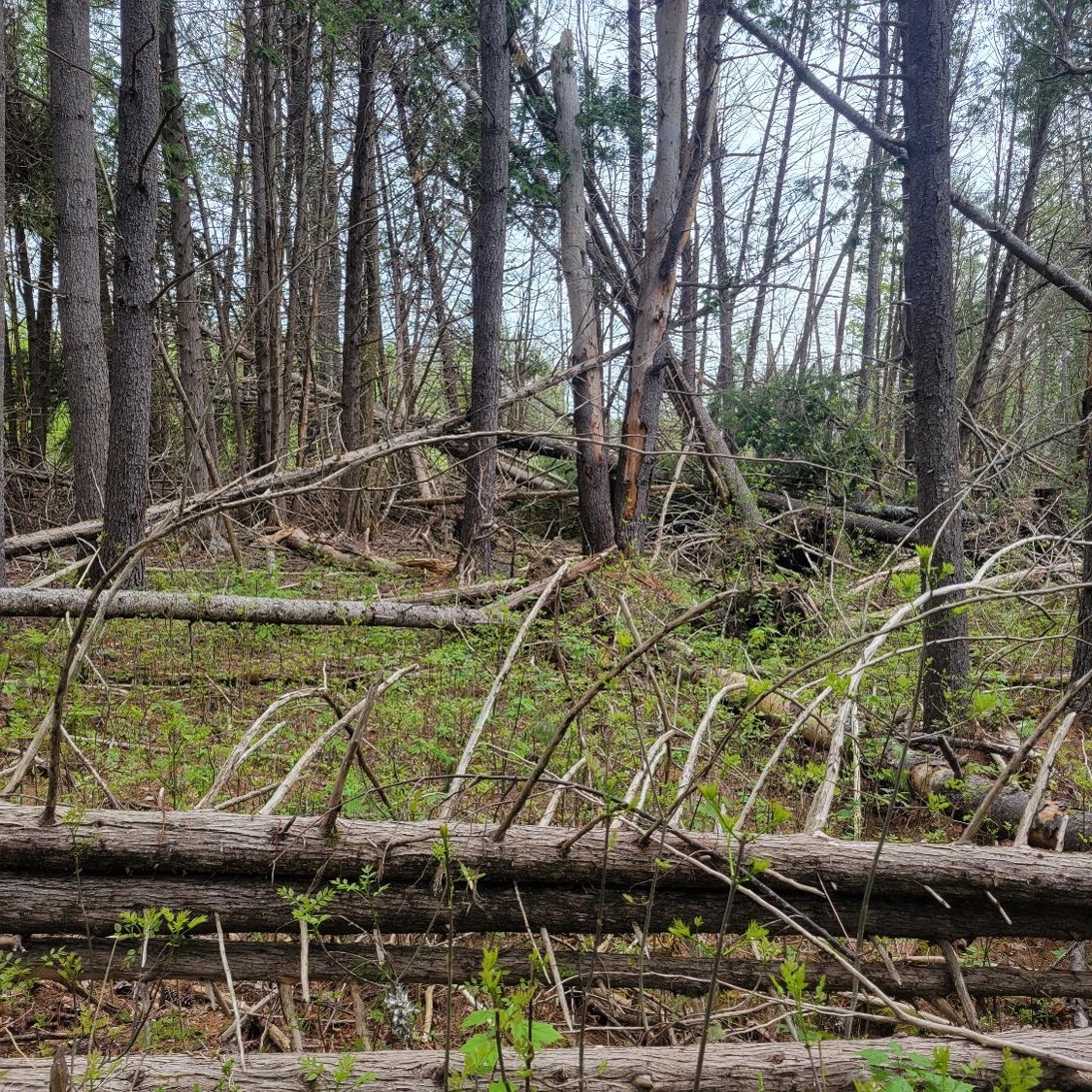
Forest growth and yield models do their best to predict what future forests will look like. The Forest Vegetation Simulator is one example model, but requires significant calibrations to obtain accurate and reliable estimates of common forest metrics like basal area, volume, and biomass. Here’s common saying at more than one meeting I’ve been a part of recently: “FVS doesn’t like to kill trees.”
I’ve written a lot about the FVS model and its projections on this blog. Most recently I described how adding previous growth to diameter and height growth modifiers can have a big impact on the model’s predictions. Calibrating the mortality component of the FVS model can also provide predictions that align with expectations.
Calibrating the mortality of FVS can help tremendously in predicting future forests. And in my experience with many of the eastern variants of FVS, more mortality needs to be added to the “out-of-the-box” predictions that FVS provides. This helps mitigate the overpredictions of common stand attributes like volume and carbon in live trees when FVS is not calibrated.
To quantify mortality, analysts need to have reliable data that allows them to understand the amount of trees that die on a regular basis and how these relate to stand conditions. These data often come from permanent sample plots, data which are all too infrequent in many forest types. Analysts can also use stocking charts or density management diagrams to understand how stand conditions relate to mortality.
This post describes the magnitude and differences when using non-calibrated “out-of-the-box” FVS predictions with versions that apply different mortality parameters in an attempt to produce a calibrated model.
Western Maine FIA data
Data were compiled from the Forest Inventory and Analysis (FIA) database from two counties in western Maine (Franklin and Oxford counties). The data used here are the same as presented in the growth calibration post mentioned previously.
Forest types are generally maple-beech-birch or spruce-fir dominated. I used the Northeast variant of FVS to simulate the most recent inventory data and ran a simulation for 100 years. A total of 294 FIA plots were run.
Calibrating FVS mortality
There are several ways to modify the mortality components in FVS, including adjusting the maximum basal area or maximum stand density index. Another approach is to add additional mortality to tree records. This is appealing because you can set which species receive the additional mortality along with their diameter limits and any other conditions (e.g., apply mortality only in the first cycle of the projection or when the stand reaches a specified age).
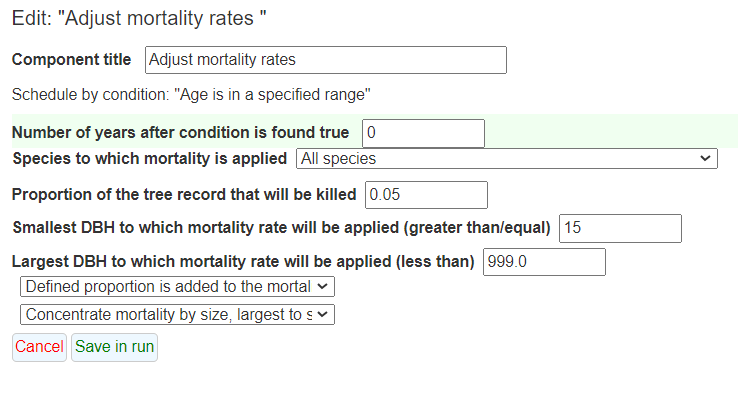
If you’re using the web application of FVS Online, additional mortality can be added under the Components tab and then clicking on Modifiers. Select Mortality Modifiers as the category and Adjust mortality rates as the component.
For this example, I added additional mortality only after the stand reaches 100 years old. The condition “Age is in a specified range” was added and applied to stands with ages between 100 and 999 years. An additional 5% of mortality was added to the tree record, from the largest-sized trees to the smallest ones. The mortality was added to all species with a minimum DBH of 15 inches:
I ran five simulations in total: one as an FVS “out-of-the-box” with no modifications and four others with additional mortality of 5%, 10%, 15%, and 20%. No management treatments or disturbances were applied to the simulations. I selected the Carbon and fuels output to look at trends in forest carbon through time.
Comparing FVS mortality modifications and out-of-the-box predictions
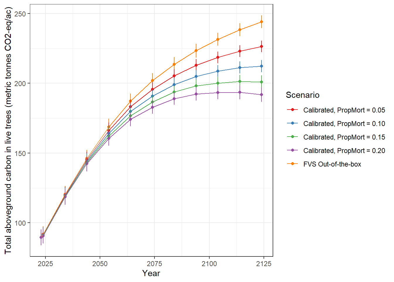
Mortality modifications to the FVS model resulted in lower aboveground carbon stocks throughout the 100 year simulation for these plots in western Maine. After 100 years, the simulation that increased mortality by 20% resulted in carbon stocks that were 22% lower than out-of-the-box predictions.
Here are the average carbon stocks throughout the simulation, with 95% confidence limits to show the variability. You’ll notice that the scenario which adds 20% mortality reaches an asymptote after 100 years, and even starts to decline slightly:
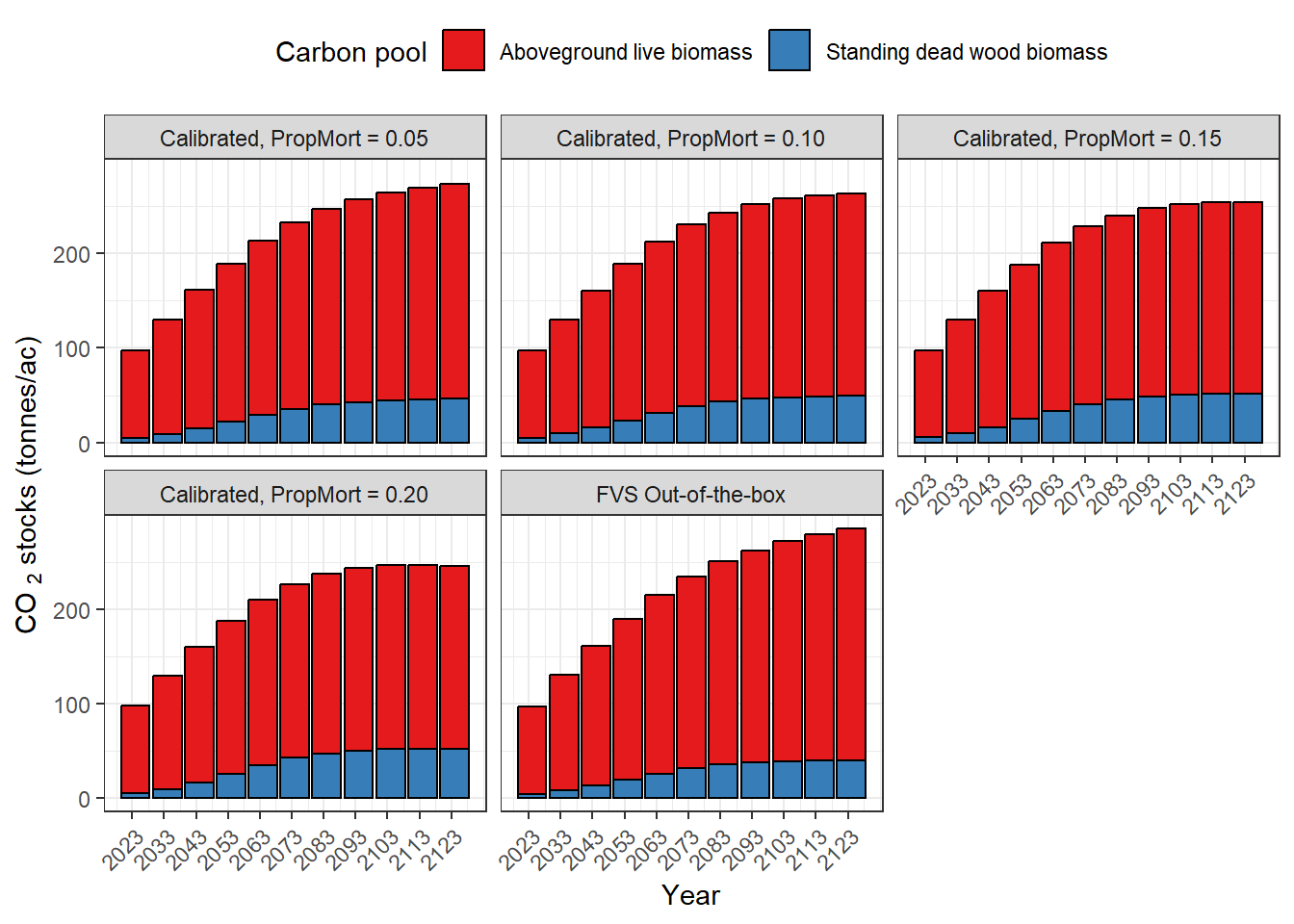
As you would expect, if you increase the mortality, you increase the number of dead trees. From a carbon perspective, this biomass transitions from the aboveground live biomass pool to standing dead (and ultimately the downed dead pool). The following graph shows these trends throughout the simulation. In particular, note the greater amount of standing dead tree biomass in the scenario that adds 20% mortality compared to the out-of-the-box scenario:
As this post shows, some relatively straightforward calibrations to the mortality component of FVS can reduce the overpredictions inherent to the model. This results in more biologically-reasonable estimates of attributes like forest carbon. Directly modifying the mortality submodels should be a go-to action for any analyst that sees predictions from FVS that seem too high.
Of course, knowing which values to set the mortality parameters to is where most of the effort on calibrations needs to be done. For this, data from permanent sample plots or stand management diagrams can be your best friend.
–
By Matt Russell. Email Matt with any questions or comments.